
")
After having spent some time on the expectation value of the the sigma observable for a product state, let's try to do the same for an entangled state.
Let's choose our entangled state to be for instance[1]:
For simplicity, let's write each composite vector as |uu> and |dd> - but still remembering that such vectors are nothing else than a tensor product of the basis vectors of each sub-space - and so simplify this equation from now on as :

Let's look first at the expectation value of Alice's σ of this state along the z-axis. We know already all the machinery we need to compute it

or
so finally
Let's look now at the expectation value of Alice's σ of this state along the y-axis

Finally, if we focus on the x-axis of the expectation value
and we are left once more with zero as result.
We could have done the same calculation for σB and we would have found the very same result.
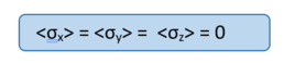
So we get a very different result than for an product state, as all σ expectation values for any observer along any axis is zero.
An expectation value equal to zero for an observable for which the eigenvalues are +1 or -1 means that there is an equal probability for each experimental outcome.
That's where lies the true weirdness of entanglement: we can know nothing a priori of the value of the subsystem, but however, if both observables are measured along the same axis, they are found to be correlated. This means that the random outcome of the measurement made on one particle seems to have been transmitted to the other, even if the distance and timing of the measurements can be chosen so as to make the interval between the two measurements spacelike, hence, any causal effect connecting the events would have to travel faster than light.
In the next article, we will demonstrate the correlation between the two sub-systems, and introduce the concept of composite observables.
[1] We verify that our state is a normalized vector, as <entangled|entangled> = 1/2 + 1/2 = 1.