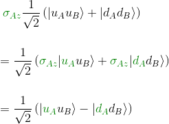
So far we have described the entangled state as this very puzzling composite state where we ignore everything about each subsystem taken separately but where the measure of one subsystem gives us direct (or real in the EPR vocabulary) information about the measurement of the other subsystem.
The previous article Expectation value of an entangled state exposed the first part: the outcome of the measurement of each subsystem is completely random. It's time now to look at the second part, the correlation.
For this, we have to introduce a new kind of observable, wider than the ones that Alice and Bob can measure separately, by using only his own detector. The measurement of this new family of observables, the composite observables, requires both detectors.
More precisely, the composite observable is an observable that is mathematically represented by first applying Alice's observable and then Bob's observable.
To make it more concrete, let's take the example of the previous entangled state

If we ask Alice to measure σAz, Bob to measure σBz and then to compare their results, that's what we have to calculate to predict the result:

We have done half the work in the previous article:

Applying now σBz, we get:
This section of the article is only available for our subscribers. Please click here to subscribe to a subscription plan to view this part of the article.
Remark 2: we said that the correlation exists when the observables are done along the same axis. We will see that even if is perfectly doable for Alice and Bob to observe together in different directions, say Alice along direction x and Bob along direction y (which is not true for the same observable, as the components x, y, and z of σ dont commute with each other inside the same space), however the product operators won't commute anymore.

