
")
In this article, our aim is to expose the teleportation algorithm introduced in The quantum teleportation algorithm but this time as implemented with Google Cirq API.
As a quick reminder, we show again the quantum circuit, and which operations/gates Bob has to apply after Alice's measurements:
Alice's measurements and Bob's operations
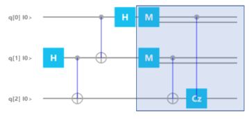
Note that after the measurement, we have classical information, which we represent in circuit diagrams with two lines (instead of one line for qubits)
To get a better idea of the possible outcomes Alice can get when she will measure, we can group terms containing the same state for the first two terms.
There are four possibilities for the first two qubits, namely |00>,|01>,|10>, and|11>. Grouping these terms together, we can rewrite the state
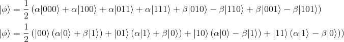
Now Alice measures her two qubits (the first two qubits).
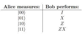
- Suppose she gets the |00> outcome. Then, Bob’s qubit is in the state α|0> +β|1>, which is |ψ> exactly. In this case, we are done, and Alice’s unknown qubit |ψ> has been teleported to Bob.
- Suppose instead Alice measures |01>. By looking at the above expression, we see that Bob’s qubit in this case would be α|1>+β|0>. This is almost |ψ>, but the amplitudes are flipped. How can we get|ψ> exactly from this state? We can perform a NOT gate X(α|1> +β|0>) = α|0> +β|1> =|ψ>.
- If Alice measures |10⟩, Bob’s qubit is in the state α|0⟩−β|1⟩. Further, he can obtain |ψ⟩ by performing a Pauli-Z gate on his qubit. As we have seen in the previous article Introduction to quantum logic gates that will have for effect to negate the |1> basis state to -|1>. That is, Z(α|0⟩−β|1⟩) =α|0⟩+β|1⟩ = |ψ⟩.
- And finally in the case of Alice measuring |11>, Bob would have to apply both the NOT gate and the Pauli-Z gates.That is ZX(α|1⟩−β|0>) =α|0⟩+β|1⟩ = |ψ⟩.
Thus, in all four measurement cases, Bob is able to obtain exactly Alice’s unknown qubit |ψ> without either knowing what the actual state is.
For summarize, we enumerate all measurement possibilities in the table below.
After the measurement, we have classical information, which we represent in circuit diagrams with two lines (instead of one line for qubits).
The controlled-X and controlled-Z are thus conditional on these measurement outcomes.
If the second qubit comes out to be a zero, then we do NOT perform an X gate on Bob’s qubit. If the second qubit does come out to be one, then we do perform an X gate.
Similarly for the controlled-Z but with the first qubit.
Quick start
You can first have a quick overview of our program by going to our github code repository here
1) If you have no Python environment installed, and still want to execute easily and quicky the python program, click here.
You will be able to open a jupyter python notebook on a remote executable environment, making the code immediately reproducible.
Once the environment is built, navigate to teleportation/cirq_teleportation.ipynb, click on Cell -> Run All.
It will first install the Cirq API (first cell), then build the quantum teleportation circuit (second cell).
To replay the program, you don't need to re-install the Cirq API. Just place yourself into the second cell and then click on Cell -> Run All Below.
2) If you have Python installed locally, you can directly clone our project and run either the Jupyter Notebook cirq_teleportation.ipynb or the Python program cirq_teleportation.py.
Cirq program to entanglement
In our previous java implementation, we have verified that Alice's qubit was actually teleported with an initial qubit initialized as:
|q0> = |1>
|q0> = α|0> + β|1> with the value α set to √3/2 = 0.866
With Cirq implementation, we are able to do better by veryfing the teleportation for any randomly generated numbers α and β.
To do this,
a) we first generate two random numbers and display the Bloch Sphere coordinates x,y, and z for this given qubit.
ranX = random.random()
ranY = random.random()
# Run a simple simulation that applies the random X and Y gates that create our message.
q0 = cirq.LineQubit(0)message = sim.simulate(cirq.Circuit([cirq.X(q0)**ranX, cirq.Y(q0)**ranY]))
# Prints the Bloch Sphere of the Message after the X and Y gates.
print("Bloch Sphere of Message After Random X and Y Gates:")expected = cirq.bloch_vector_from_state_vector(message.final_state, 0) print("x: ", np.around(expected[0], 4), "y: ", np.around(expected[1], 4), "z: ", np.around(expected[2], 4))
b) in a second time, we use exactly the same numbers for Alice's first qubit, apply the quantum teleportation circuit, and compare the measure of Bob on the Bloch Sphere with the measurements of a).
circuit = make_quantum_teleportation_circuit(ranX, ranY)
def make_quantum_teleportation_circuit(ranX, ranY):circuit = cirq.Circuit()msg, alice, bob = cirq.LineQubit.range(3)
# Creates Bell state to be shared between Alice and Bob.circuit.append([cirq.H(alice), cirq.CNOT(alice, bob)])# Creates a random state for the Message.circuit.append([cirq.X(msg)**ranX, cirq.Y(msg)**ranY])# Bell measurement of the Message and Alice's entangled qubit.circuit.append([cirq.CNOT(msg, alice), cirq.H(msg)])circuit.append(cirq.measure(msg, alice))
# Uses the two classical bits from the Bell measurement to recover the# original quantum Message on Bob's entangled qubit.circuit.append([cirq.CNOT(alice, bob), cirq.CZ(msg, bob)])
return circuit
c) Finally, we print the circuit and check that the two Bloch Sphere coordinates generated from the same random state are identicial
Circuit:
0: ───X^0.321───Y^0.978───@───H───M───────@───
                          │       │       │
1: ───H─────────@─────────X───────M───@───┼───
                │                     │   │
2: ─────────────X─────────────────────X───@───

Bloch Sphere of Message After Random X and Y Gates:
x:  0.0363 y:  -0.8453 z:  -0.5331

Bloch Sphere of Qubit 2 at Final State:
x:  0.0363 y:  -0.8453 z:  -0.5331