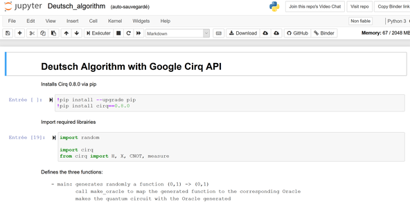
This article will walk through on how to implement the Deutsch algorithm introduced in our previous article The Deutsch-Jozsa algorithm with Google Cirq software library.
Quick Start
You can find all the technical details on how to run this program at this adress: https://github.com/cyrilondon/quantum-mechanics-python/tree/master/deutsch.
The good news is that you don't need any python environment installed on your computer: by following the instructions, you will be able to run the program on your favourite browser (via Python Jupiter notebook).
Run the program (either by clicking Cell -> Run All the first time or just by cliking the last cell afterwards) and you will see the quantum circuit randomly generated (corresponding to a random function to evaluate) as well as the result (0 or 1) of the measurement.
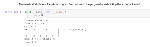
In this case, the program chose randomly the function f(x) = 1 to be evaluated (<1,1> means <f(0)=1, f(1)=1) , and measured the final state of the first qubit as 0, as expected (f(x)=1 means f is constant and thus 0 should be measured).
The Program
We recall from our last article the quantum circuit corresponding to the Deutsch algorithm
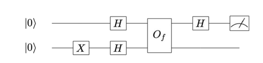
Its implementation in Cirq syntax is described in the make_deutsch_circuit function below
def make_deutsch_circuit(q0, q1, oracle):
c = cirq.Circuit()
# Initialize 2 qubits.
# Apply Hadamard gate to first qubit and NOT + Hadamard to the second
c.append([X(q1), H(q1), H(q0)])
# Append quantum oracle.
c.append(oracle)
# Apply Hadamard to the first qubit and measure in X basis.
c.append([H(q0), measure(q0, key='result')])
# Return circuit
return c
The most important part of the program concerns of course how the four distinct quantum Oracle (corresponding to the four functions to be evaluated) are implemented.
Let us consider the Cirq function responsible of generating those Oracles
#Pick a secret 2-bit function and create a circuit to query the oracle.
secret_function = [random.randint(0, 1) for _ in range(2)]
oracle = make_oracle(q0, q1, secret_function)
def make_oracle(q0, q1, secret_function):
#Gates implementing the secret function f(x).
#f(0)=1
if secret_function[0]:
yield [CNOT(q0, q1), X(q1)]
#f(1)=1
if secret_function[1]:
yield CNOT(q0, q1)
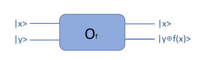
As a reminder, the oracle maps the state 


We recall as well the final state in which we should be just before the final measurement of the first qubit
which could be broke down in the four following cases

Case f(x) = 0
We notice that in case of f(x)=0, the make_oracle routine does not return any Oracle (the two if statements are evaluated as false), as expected. Indeed, if f(x)=0
so that we |x> stays in its original state 1/√2(|0> + |1>) leading to a measurement of 0.
The output of the program would be in this case as per below

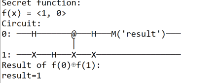
Case f(x) = x
Another trivial Oracle to find out is for the case f(x) = x.

Actually if f(0) = 0 and f(1) = 1 the the make_oracle routine only goes through the second if statement and returns the CNOT gate as for the quantum Oracle.
Also, let us double check that the final state of first qubit after the CNOT gate is 1/√2(|0> - |1>) leading to a measurement of 1.
We are all good, i.e the state of the first qubit is the one expected as per the table above.
If you are more into matrix representation, you may wish to follow this path rather
And the result printed out by our program looks like
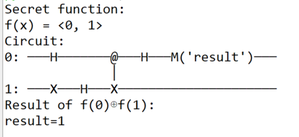
Case f(x) = Not(x) => f(0) =1, f(1) = 0
If f(0)=1 and f(1)=0, the function goes through the first if evaluation only, which yields to the following quantum circuit [CNOT(q0, q1), X(q1)]
As per above, we should verify that the quantum circuit transforms the first qubit's state to -1/√2(|0> - |1>), leading to a measurement of 1.
Compared to the previous quantum circuit, we just have to apply an extra Pauli-X gate to the second qubit, which yields to:

And the state of the first qubit is -1/√2(|0> - |1>), as expected.
Case f(x) = 1
FInally, the last case to consider is when f(x)=1.
In this particular case, the make_oracle routine goes through the two if statements, leading to the following quantum circuit
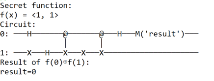
Compared to the previous quantum circuit, we just have to apply an extra CNOT gate to the second qubit's state leading to:
The state of the first qubit after the Oracle is applied is -1/√2(|0> -+|1>), as expected.
CQFD.